Perplexity DeepSeek MoE

Speaker: Lequn Chen

Sources

• https://www.perplexity.ai/hub/blog/lower-latency-and-higher-throughput-with-multi-node-deepseek-deployment
• https://github.com/ppl-ai/pplx-kernels

1. Setup

Multiple nodes to serve a single Deepseek instance (not DP with multiple replicas)

• Good for MoE models like Deepseek V3/R1
• In most systems, latency and throughput are often conflicting goals. Examples:
  • dense models: batch size++ means throughput++ and latency++
  • TP in a node: reduce compute per GPU → latency–; decreases # replicas → throughput–
• MoE models can achieve both higher throughput and lower latency when utilizing more GPUs in multi-node deployments

Latency ↔ user experience

Throughput ↔ your cost

It’s almost necessary to do disaggregated prefill on Deepseek models.

• P and D can have very different setups
• P and D are implemented in different code paths

We only consider D here

D is memory-bound workload, so the most important factor is batch size. P and D length doesn’t really matter

2. Baseline: single-node deployment

Hardware: 8xH200

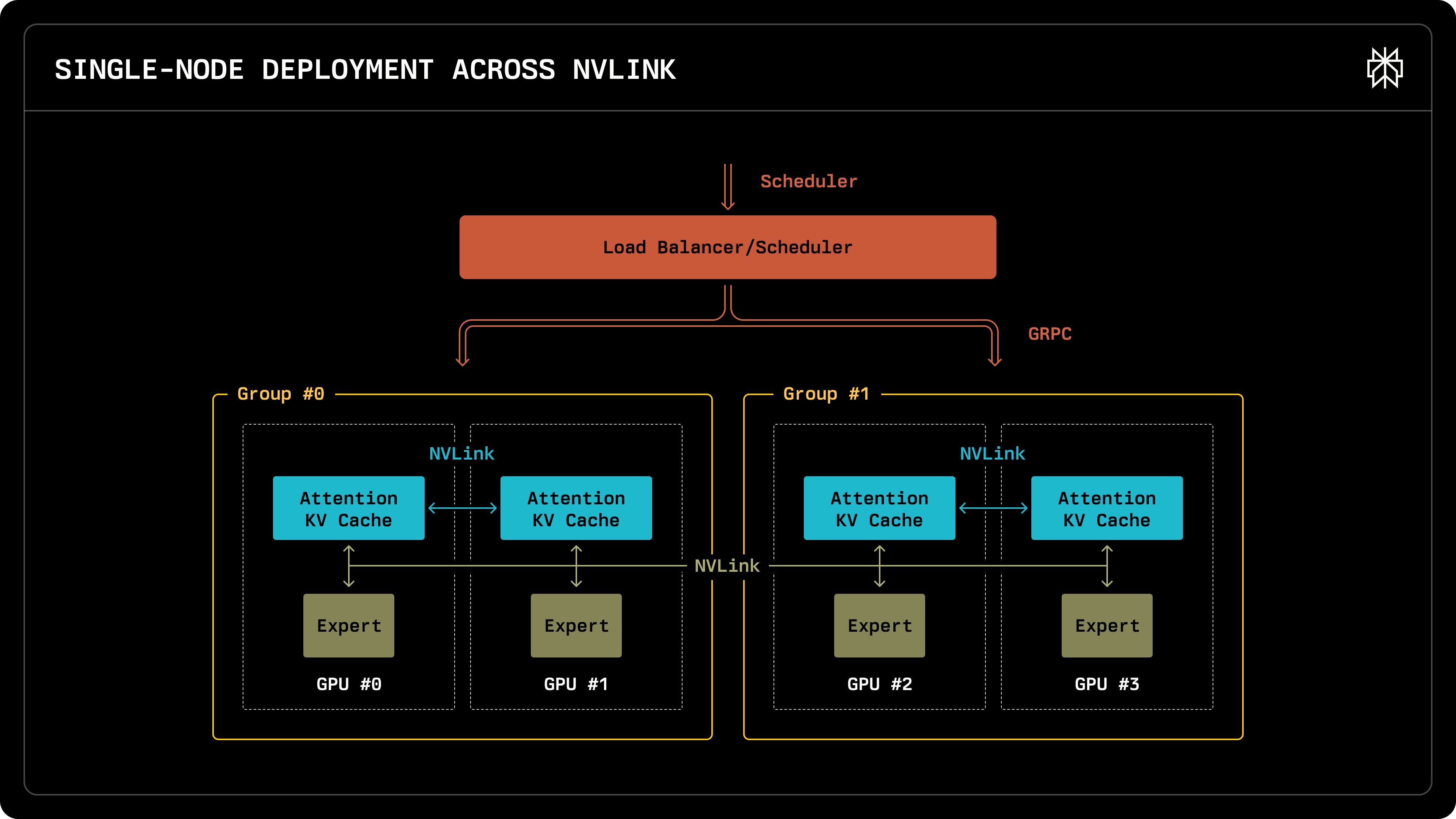
• Load balancer: distribute requests to DP groups (model replicas) using gRPC
  • not like nginx that supports 1M qps
  • reasonable LLM inference qps is <1k
• Each DP group maintains its own attention KV cache
• GPUs are connected via NVLink → communication is fast
• All DP ranks share the same experts

Can Deepseek fit into a single node (8xH200)?

• DeepSeek is 671B; 1xH200 is 141GB
• using EP8 DP8 TP1, model uses 100GB per H200
• 40GB left as KV cache per H200
• one token is ~70KB KV cache. if one request is 5k tokens, each GPU can hold 100 requests
  • 40GB / 70KB per token / 5k tokens per request = ~100 requests

3. Multi-node deployment

Hardware: multiple 8xH100 nodes

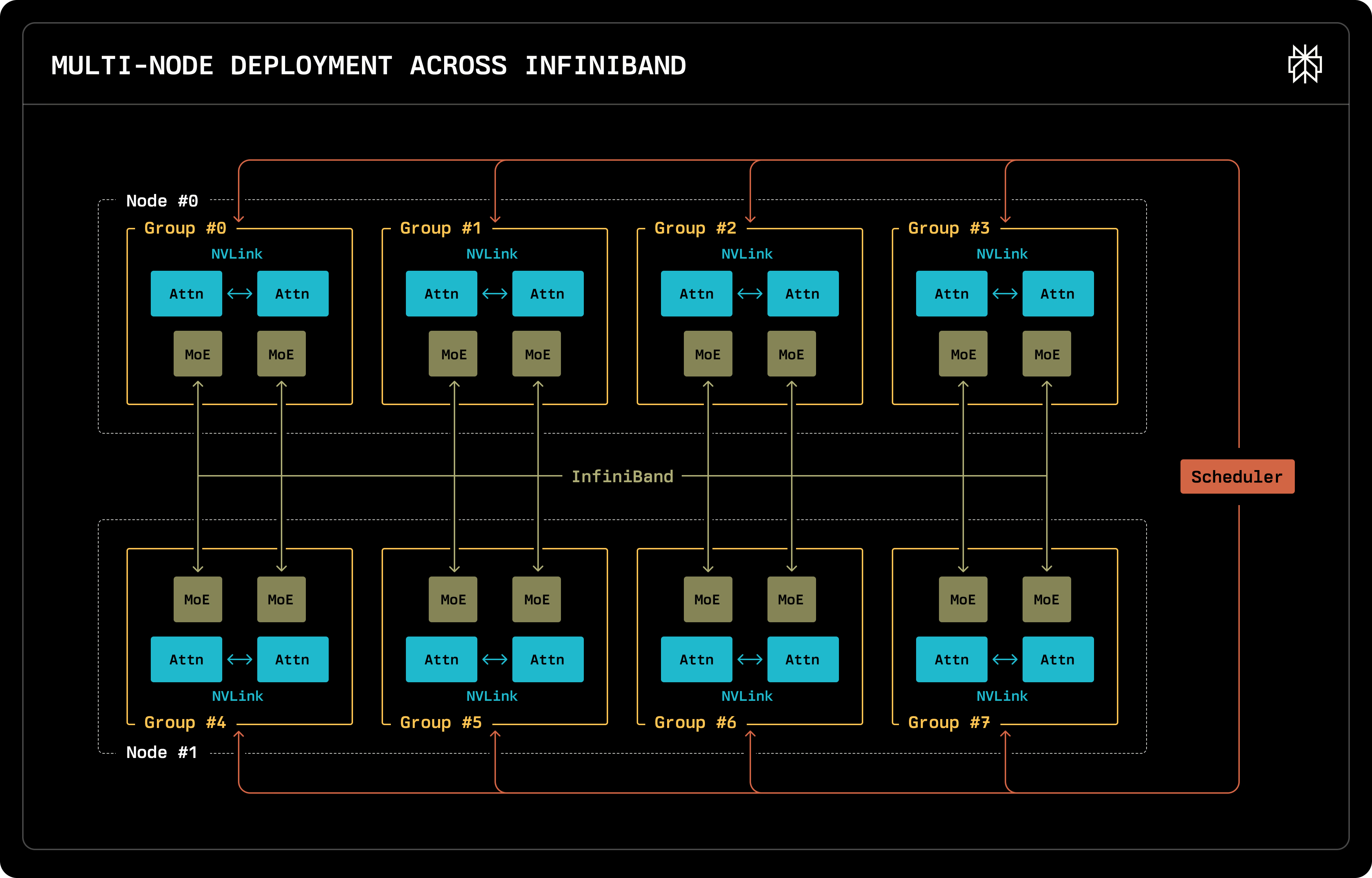
• Attention under TP are connected via NVLink
• Experts across nodes are connected via InfiniBand

4. Deepseek MoE parallelism

https://www.perplexity.ai/hub/blog/efficient-and-portable-mixture-of-experts-communication

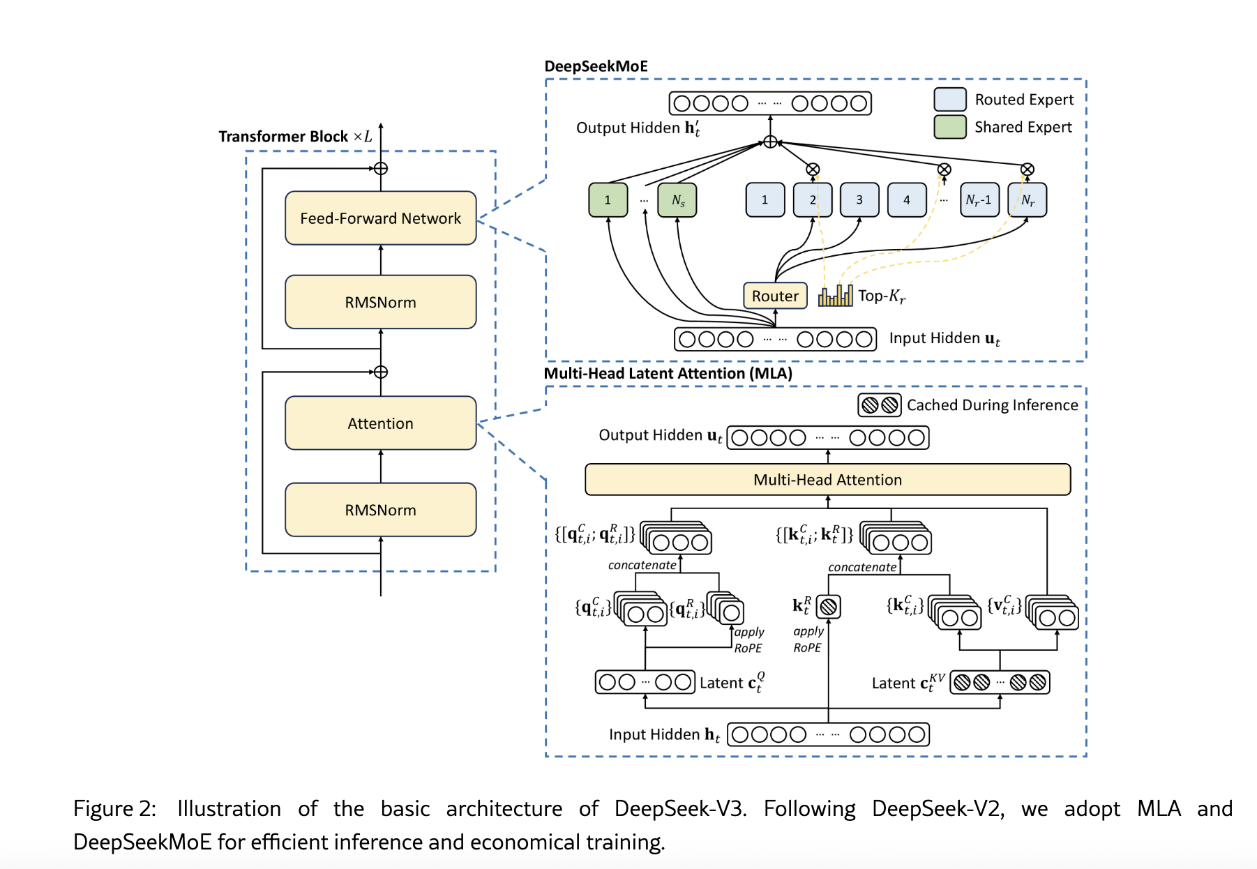
EP (MoE part)

• MLP is replaced with DeepSeekMoE (256 routed Es + 1 shared E)
• Most model weights are for Es, not Attention.
• So in multi-node deployment, we basically shard Es
• Routed Es are distributed evenly. Example: 128 GPUs → 2 Es per GPU
• The shared E is replicated
• Before E compute, GPUs perform AllToAll ops to dispatch tokens
• After E compute, another AllToAll to accumulate results

DP (MLA attention part)

• Attention weights are replicated among DP groups
• Different DP groups receive different requests
• Why DP for MLA? → Cannot split into (for example) 128 parts

TP

TP for dense models

• shard Linear Projections along row or column
• shard Attention along the attention head

TP for DeepSeek MLA

• MLA first uses kv_a_proj to compute the latent vector, then uses kv_b_proj to transform it into the space of each attention head
• the latent vector is shared by all heads
  • all TP ranks replicate kv_a_proj and kv_b_proj
  • MLA stores the latent vector in the KV Cache. Each TP rank stores an identical copy of the KV Cache.
• TP still provides partial compute reduction
• TP slightly saves more memory space: some kv projection can be split
  • why “slightly”: most weights are on the MoE part
• EP = DP * TP

EP + DP

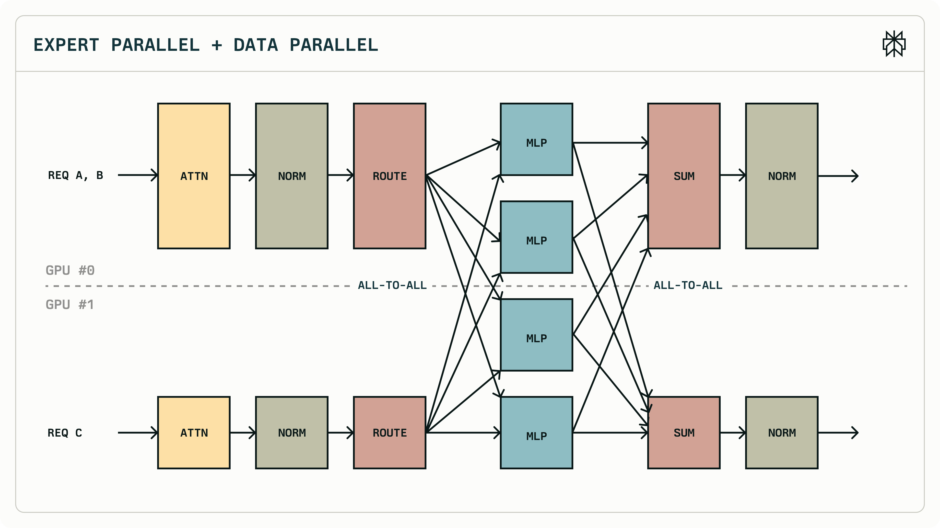
• GPU0 is DP group1; GPU1 is DP group2
• ATTNs are computed independently; Es are shared

EP + TP

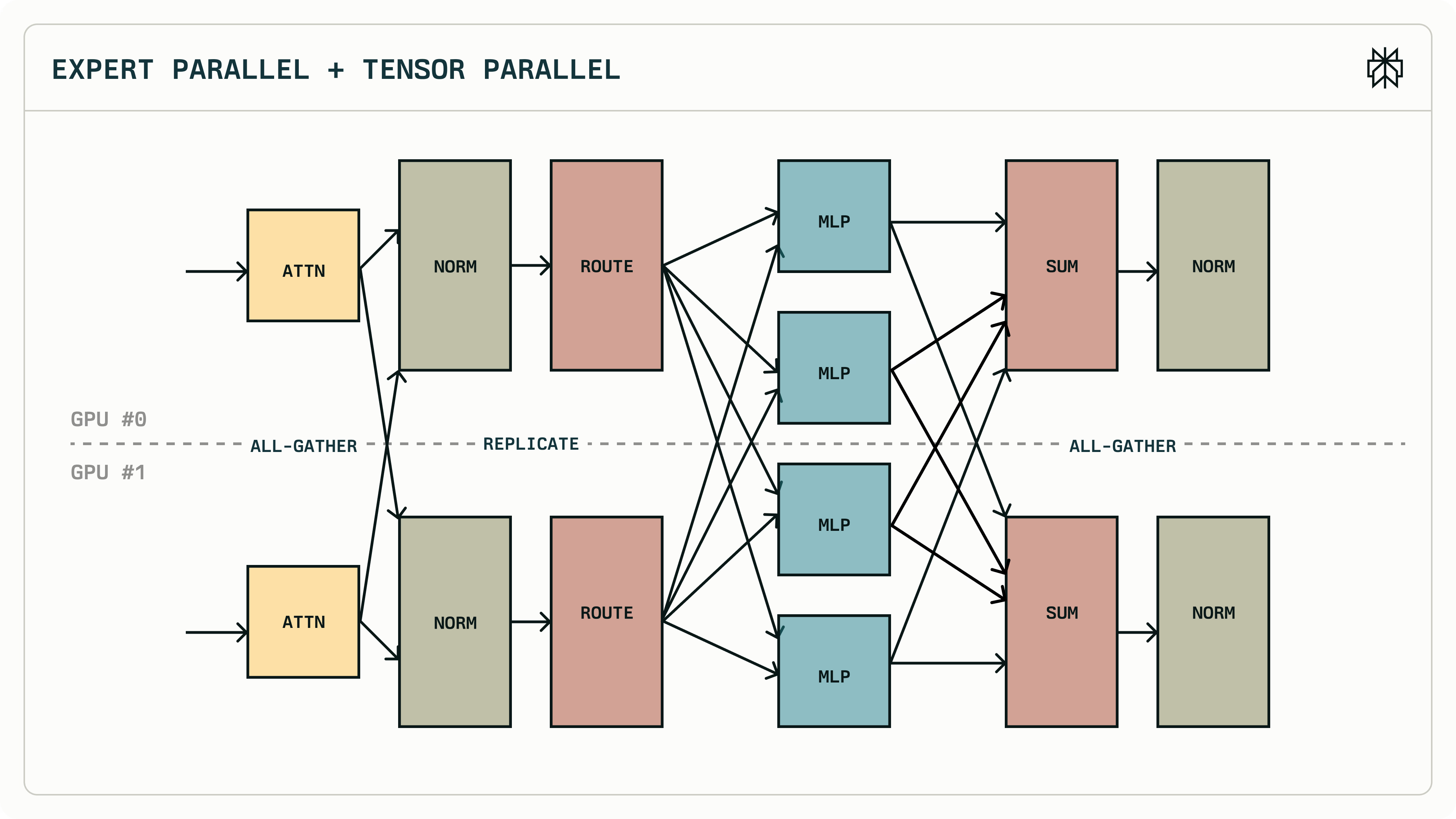
• ATTN part is sharded. Needs AllGather (replicated) or AllReduce (reduced) to combine results
• Es are still shared

Traditional TP in Megatron-LM

• MLP: A is split column-wise; B is split row-wise
• Attention: split among attention heads

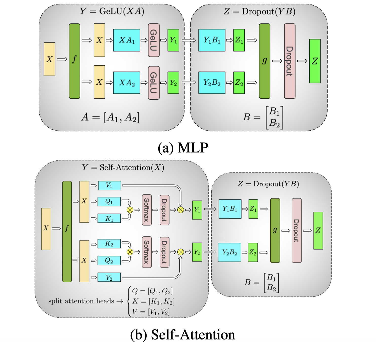
Blocks of Transformer with Model Parallelism. f and g are conjugate. f is an identity operator in the forward pass and all reduce in the backward pass while g is an all reduce in the forward pass and identity in the backward pass.

5. Single vs Multi-Node

setup

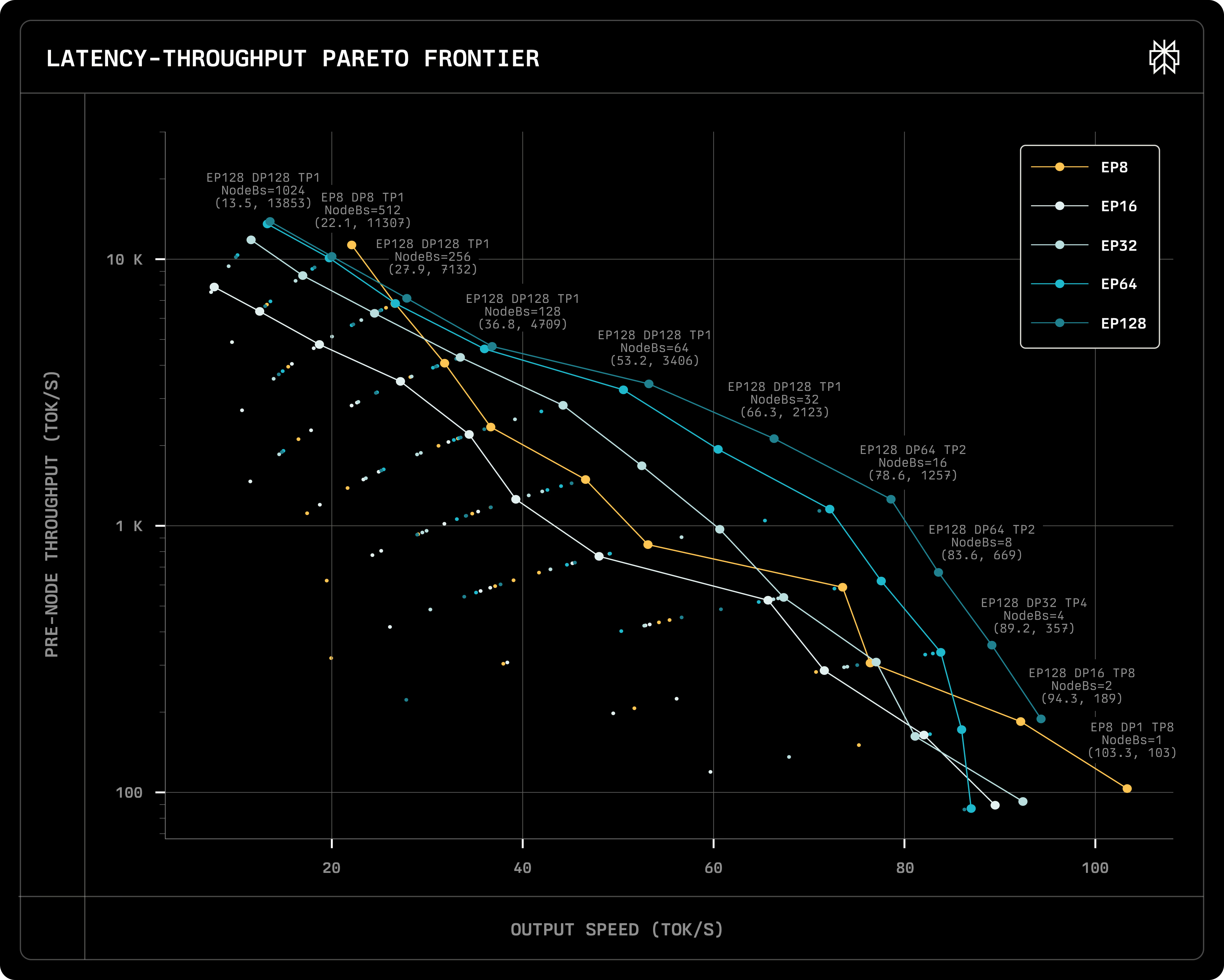
throughput vs latency under single-/multi-node

• x-axis: user perceived generating decoding speed (tok/s)
• y-axis: PER NODE throughput (tok/s) in log scale → can be converted to cost ($ per million toks)
• setups: nodes = 1, 2, 4, 8, 16 (i.e., EP=8, 16, 32, 64, 128); TP = 1, 2, 4, 8; batch size = 1, 2, 4, 8, 16, 32, 64, 128
• one data points ↔ one specific setup combination

pareto frontiers

points on the line: pareto frontiers for each EP setup

• given the same x, it gives the best y
• given the same y, it gives the best x
• we only choose pareto frontiers to deploy based on our x-y tradeoff

single-node

The rightmost yellow point (max output speed)

• EP8 → deployed on a single node; DP1 → one DP group; TP8 → shard attention to 8 parts; NodeBs=1 → one request on the node
• why fastest?
  • Attention is fast: TP8 → attention compute is split
  • MoE is fast: single node → no inter-node communication
  • batch size = 1 → only 37B activated → memory need is not too big

Points on the yellow line: batch size++ → y++ and x–

Compared to other lines, when batch size increases, latency decreases more dramatically on the yellow line

• when NodeBs=1, only 37B are activated
• when NodeBs>1, more weights are activated, and the performance will be limited by the memory bandwidth of a single node

multi-node

with more nodes (i.e., larger EP), we have better results (excluding the yellow line → no inter-node communication)

• we achieve better latency and throughput at the same time!

scalability

Q: in real workloads, batch size is dynamic
- then your x-y will move on the EP line

sub-linear scalability on a single node: when NodeBs x 8, the throughput won’t be 8x (e.g., only 2x)

• bottleneck is on loading Es

horizontal scalability on more nodes: with EP=128, each node only holds 2 experts, this time throughput is more proportional to NodeBs

• istribute your batch size on more nodes → aggregated bandwidth is larger
• one metric to estimate the scalability is, # of experts to read each time / # of experts stored on this node. if this metric is larger, the scalability is better
  • EP8 DP1 TP8 point: the single node reads one expert each time, and it stores all the experts → this metric is very low → sub-linear scalability
  • why? is that due to arithmetic intensity?

single-node vs multi-node

When NodeBs=128, single node has very good performance (better than multi nodes) → the current inter-node communication implementation is not good

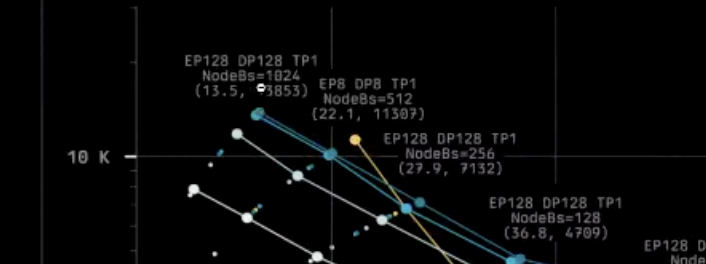
• Perplexity’s EP128, DP128, TP1, NodeBs=1024 result is (13.5, 13.8k), while Deepseek’s is (20, 15k)

you need large batch size to achieve good GroupGEMM performance

5. EP load balancing

Question: if Es are imbalanced among nodes, will it affect the pareto frontiers?

• Deepseek’s solution: replicate Es on nodes
• Expert Parallelism Load Balancer https://github.com/deepseek-ai/EPLB
  • hotter Es are put on more nodes
  • replica placement is adjusted every 5 or 10 minutes

Classical system techniques: replicating, sharding, batching, caching, scheduling, pipelining

6. Compute/communication overlapping

5-stage pipeline

• GPUs are idle during MoE Layer communication, and Infiniband is slow.
• Without overlapping: the “dispatch” and “combine” in the figure below takes a long time.
• Overlap dispatch: put the shared E computation between “dispatch send” and “dispatch receive”. Only 1~2 loc changes.
• 5-stage pipeline (from deepseek)
  • split one batch to microbatches
  • when one microbatch is doing GPU compute, the other can do MoE communication

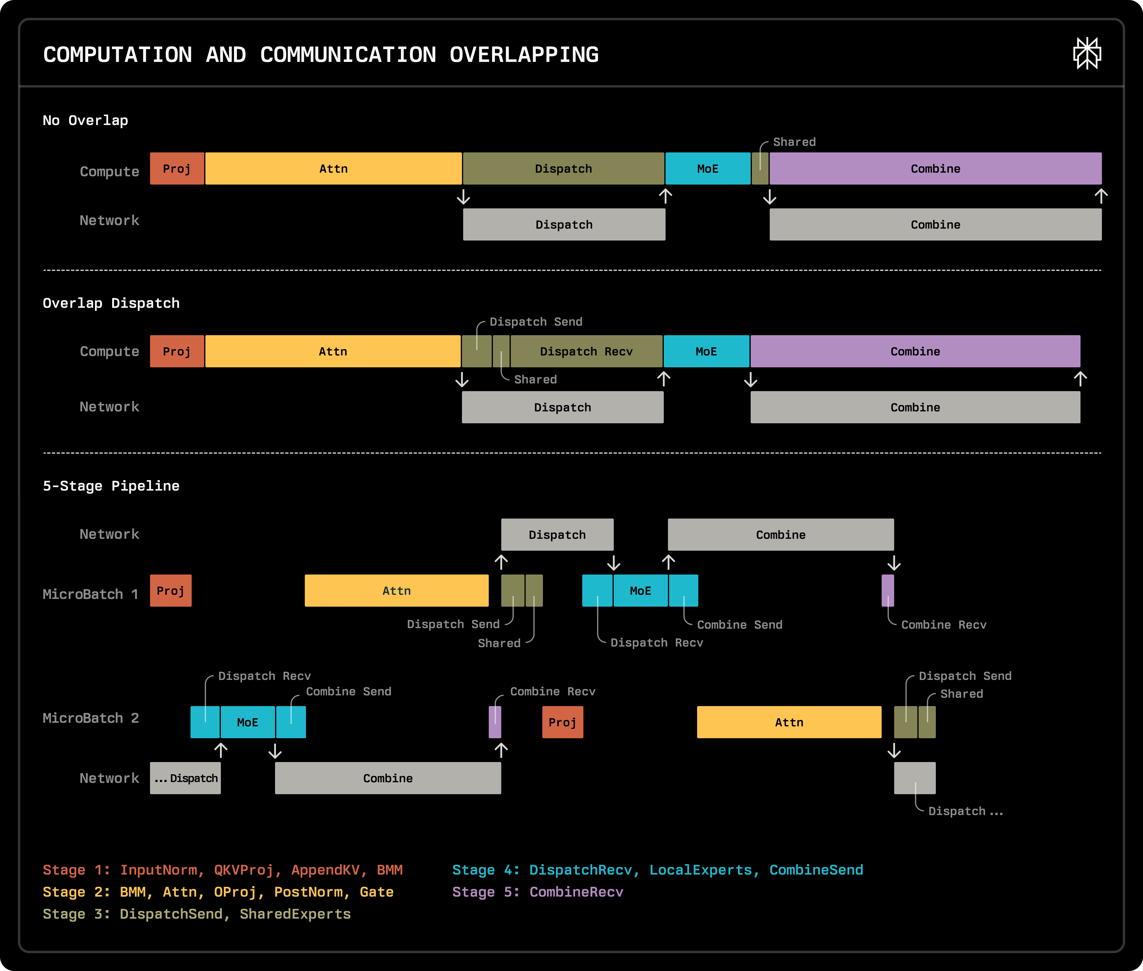
implementation

Before, Proj and Attn are in the same torch.nn.Module. now we can split them to different stages

Q: how are stages implemented? yielding ops or hardcode the workflow in a larger script?

• solution1: save intermediate results from proj (manually maintaining a state machine). This was Lequn’s initial implementation.
• solution2: use python’s yield. This was the modified implementation.
  • Will yield impact the CUDA graph? No. It’s a static execution.

Q: are you using two CUDA streams?

• one stream is enough. two microbatches in the figure has no overlapping computation

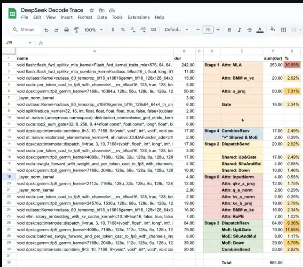
Deepseek trace

https://github.com/deepseek-ai/profile-data

• Decoding: EP128, TP1, and a prompt length of 4K (closely matching the actual online deployment configuration), with a batch size of 128 requests per GPU.
• The all-to-all communication during decoding does not occupy GPU SMs

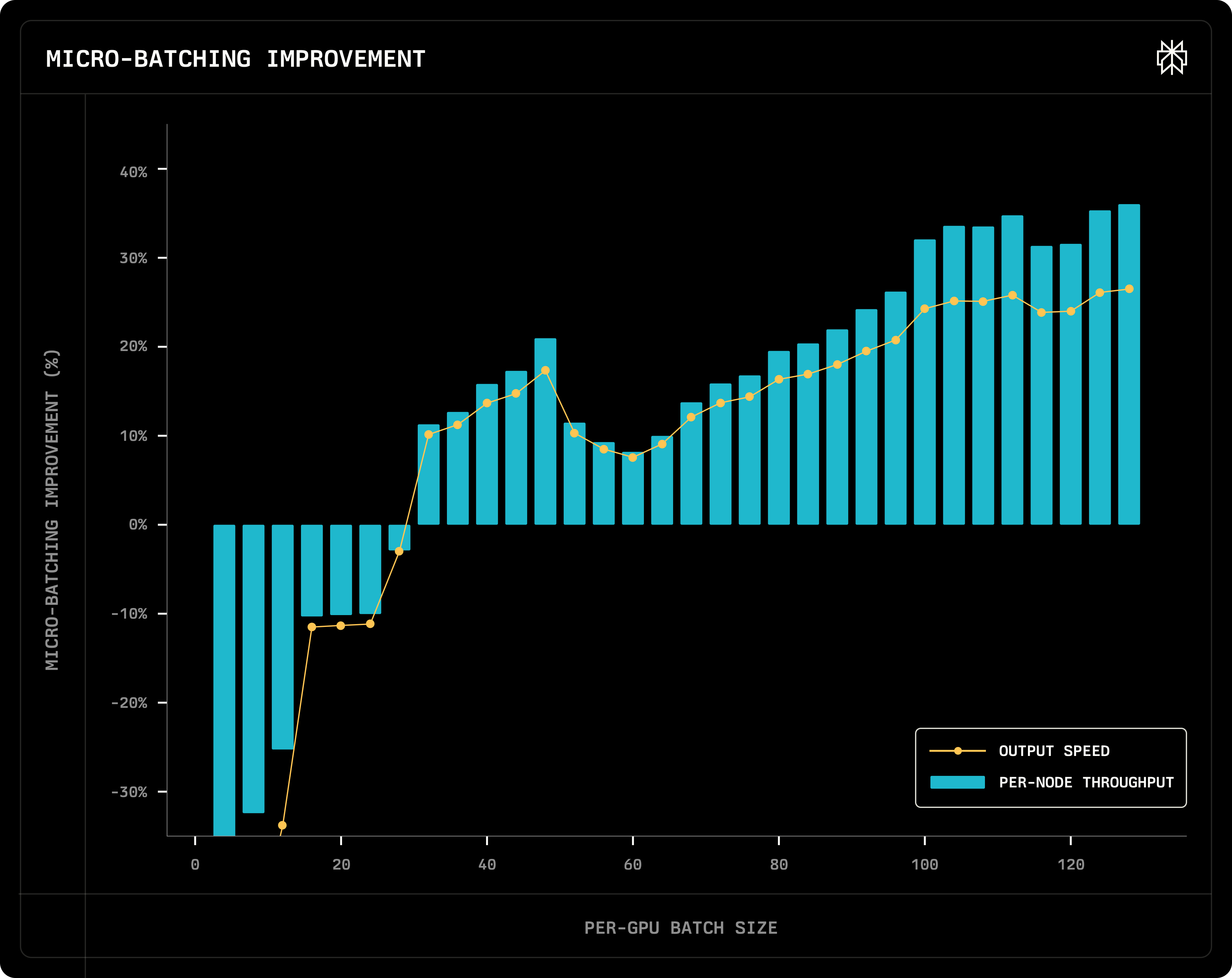
Micro-batching improvement

When batch size < 32, micro-batching harms the throughput

• why not always improving? → micro-batch size = batch size / 2 → each kernel’s computing efficiency is worse → need large enough batch size
• why 32 is the current turning point? the current communication implementation is not very good

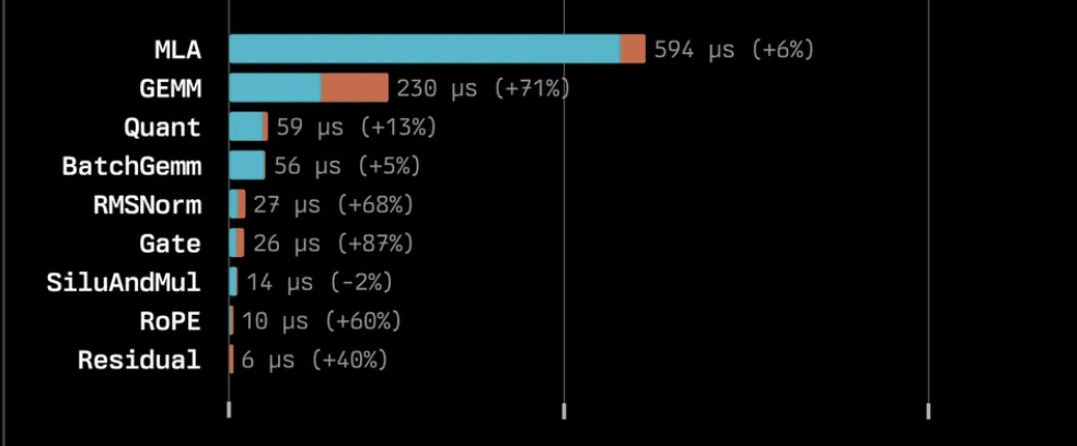
7. Layer latency breakdown

Total: w/ micro-batching, EP128 communication latency is hidden, and the total latency is reduced a lot (still slightly worse than EP8)

Dispatch: compared to EP128 No Overlap, EP128 Dispatch Overlap saves the shared E time

Perplexity vs Deepseek kernel latency: Perplexity’s multi-node implementation on infiniband is 1x slower than Deepseek’s implementation (DeepEP)

GroupGEMM (i.e. MoE computation): GroupGEMM latency is the most important metric to show that multi-node is better than single-node. multi-node → larger batch size → better performance

Kernel latency percentage

• communication (dispatch/combine) is the slowest part
• MLA latency is already the secondary slowest w/ context length = 54k. w/ larger context length, it will be worse
  • one reason is that the current batch size is very large, which requires a lot of KV cache loading

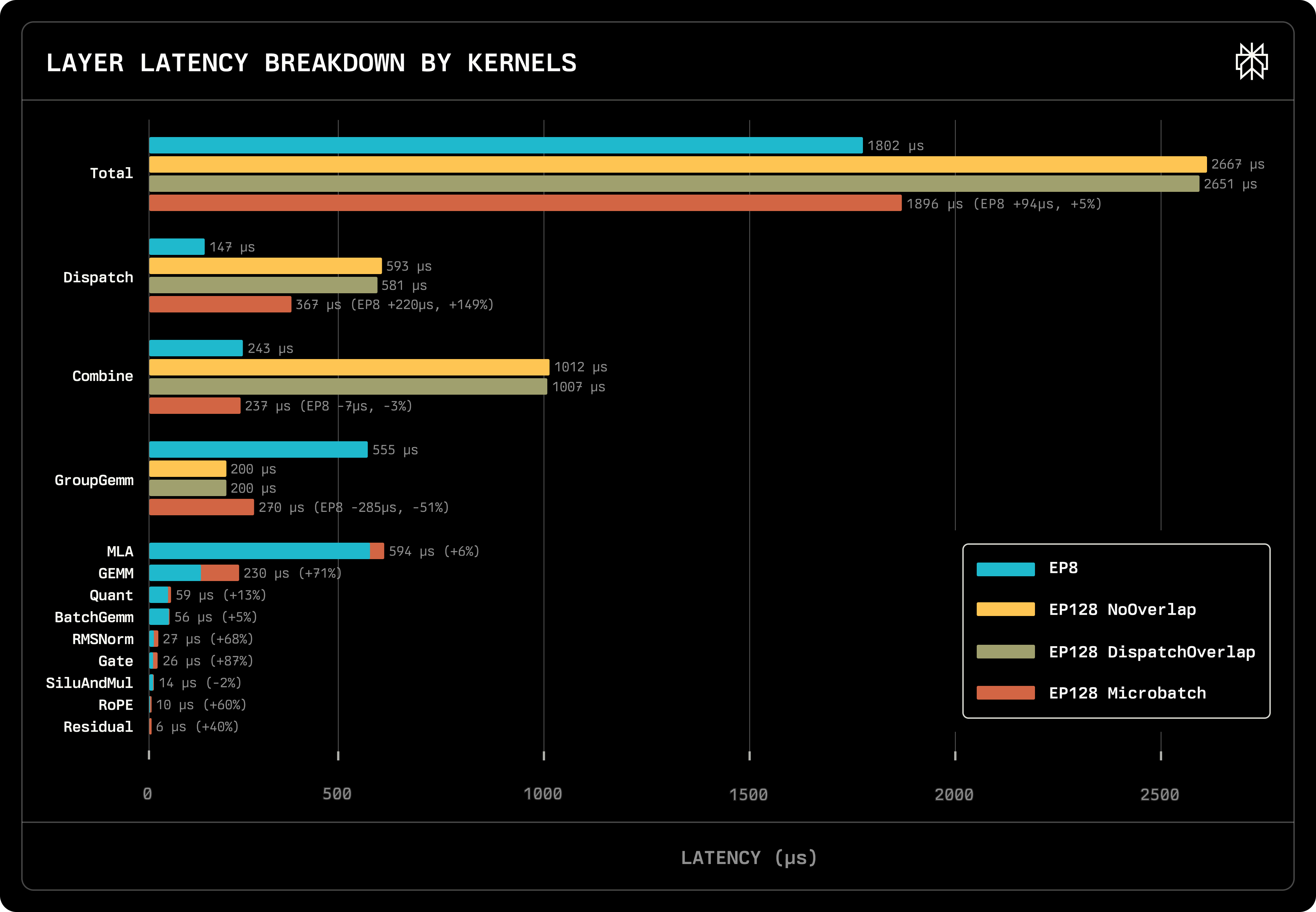
The following part is to show that micro-batching indeed is slightly slower.

GroupGEMM’s benefit is greater than the latency increase here

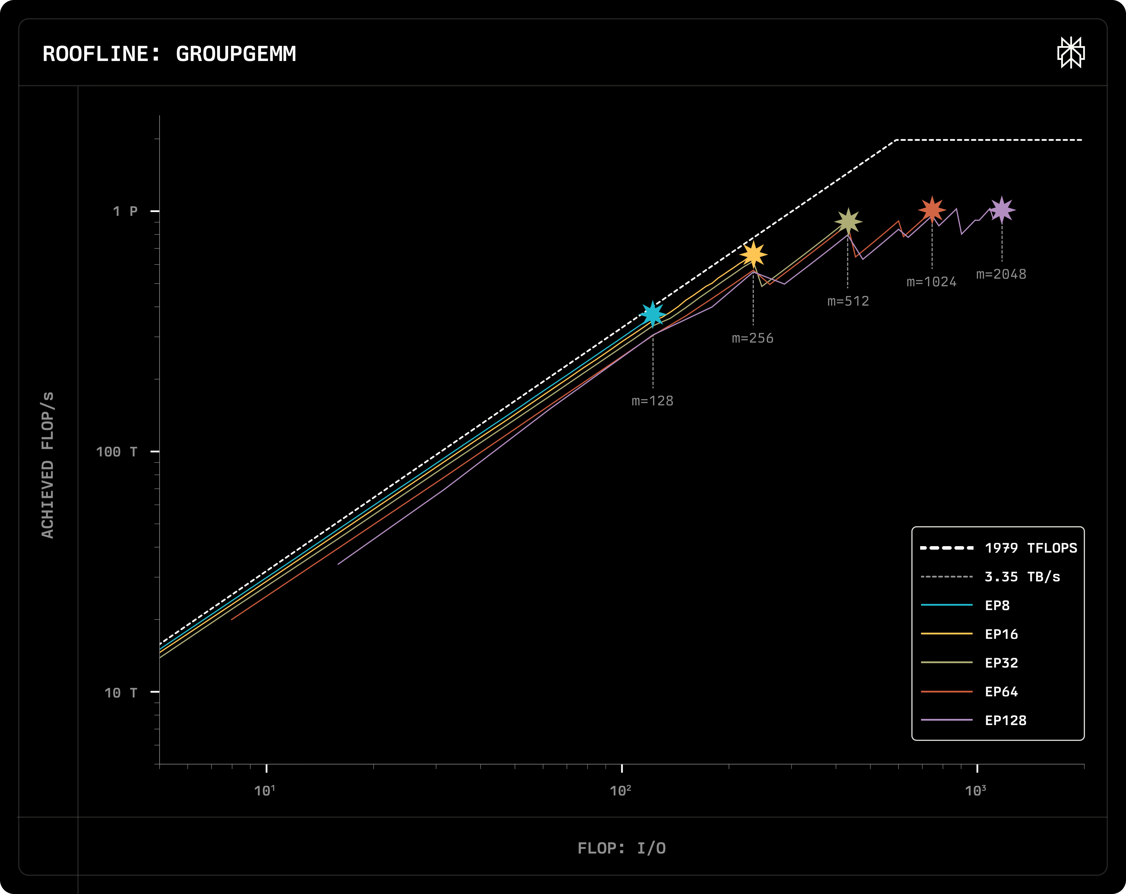
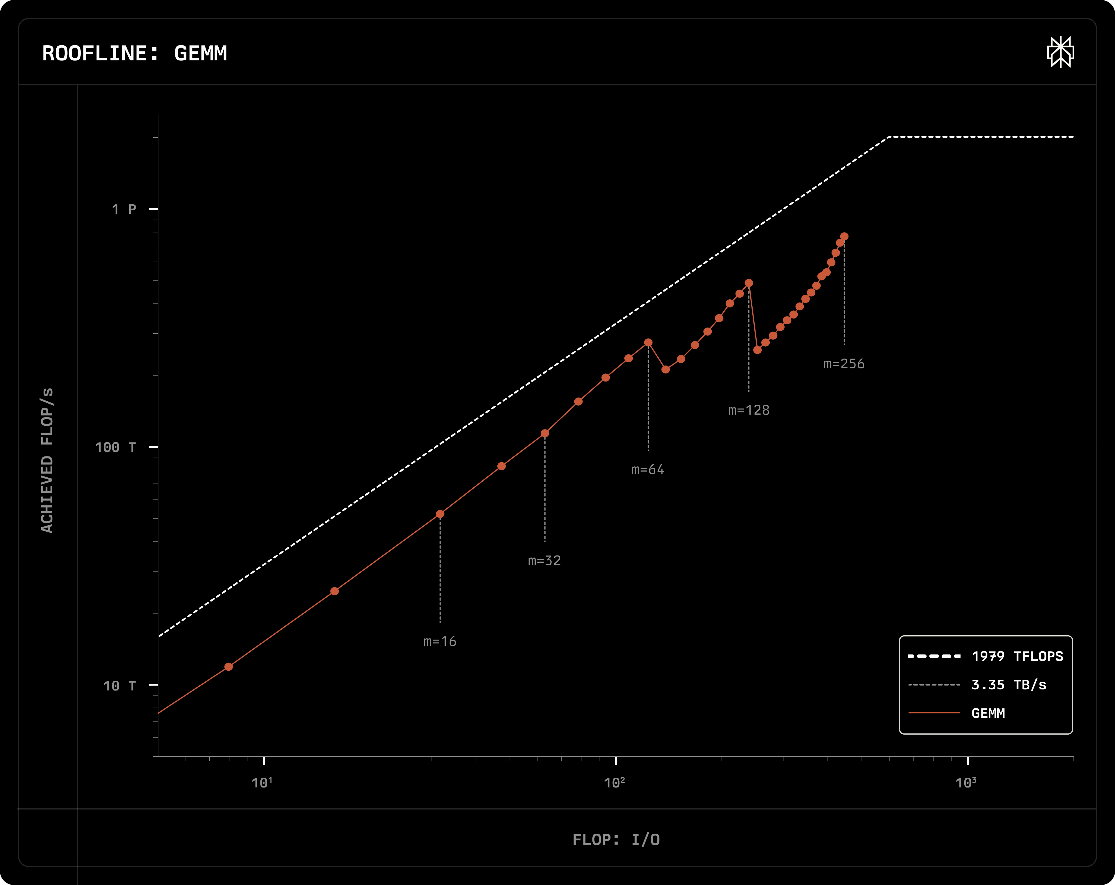
8. Roofline analysis

• Its horizontal axis is Arithmetic Intensity, the ratio of FLOP to memory I/O bytes.
• The horizontal axis value can be calculated directly from the kernel’s semantics.
• The vertical axis represents achieved performance, calculated by dividing FLOP by benchmark latency.
• The closer your implementation is to the white dotted line, the better your implementation is.
• Slope of the white dotted line: memory bandwidth.

GroupGEMM

• The implementation is from Deepseek’s DeepGEMM
• The figure shows lines of different group numbers. Example: EP8 → 256 / 8 = 32 groups
• Dots on the line represent different batch sizes. Larger batch size gives you better performance.

GEMM

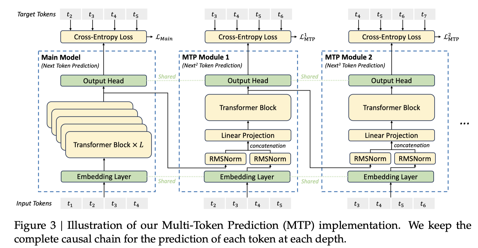
9. Multi-Token Prediction (MTP)

• MTP Module inputs: main model hidden states + predicted tokens
• We can use the MTP module to do spec decoding.
• This is a very important optimization.
  • This blog uses MTP=2. The original implementation used MTP=1 and the performance was bad.

10. CUDA graph

CUDA graph: a static computing workflow.

• input/output buffers’ pointer must be fixed
• kernel launching parameters must be fixed
• tensor shapes must be fixed

How to put MoE computations into CUDA graph?

• torch.all_to_all_single() requires all GPUs to use the same batch size
• After implementing their own AllToAll Kernel, they no longer require all GPUs to use the same batch size.

11. Future Work

The most important next optimization is Prefill Disaggregation.

The Prefill phase and Decode phase of the DeepSeek-V3/R1 model have very different computational characteristics.

Both can use different optimization strategies and deployment schemes.

• E.g., different EP configuration

QA

1. Any implementation for training?
   • This work is mainly for inference. You can go check FSDP/ZeRO
   • Training workload is good for MoE, because the amount of data is large enough.
2. Deepseek R1 w/ quantization can be deployed on a single 8xH100 node
3. Q: what are GroupGEMM’s dimensions [# activated Es on the GPU, # requests on the GPU]?
   • It should be [# Es on this GPU, 8*n/256] (ideal case where Es are tokens are evenly distributed)
   • 8*n/256 is the average # tokens per E
     • n is the batch size
     • each token activates 8 Es
     • there are 256 Es in total
4. Are decoding optimizations more algorithm-wise or system-wise?
   • spec decoding is both (but more algorithm-wise)
   • quantization is more algorithm-wise, with some system insight
     • GPU may optimize for specialized format
     • 4090/5090 GPU optimizes INT4, while H100 does not
     • B100/B200 optimized FP4
5. What is the kv cache hit rate in production?
   • Check out character.ai’s blogs
     • https://research.character.ai/optimizing-inference/?ref=blog.character.ai
     • https://research.character.ai/optimizing-ai-inference-at-character-ai-part-deux/
   • Check out mooncake’s paper
   • Highly related to KV cache capacity → single GPU is not good; KV cache offloading is important
6. Computing power increases 1.3x per year, while memory bandwidth increases 1.2x per year. → Memory-bound operator will be more and more compute-bound.

Source

https://www.youtube.com/watch?v=UMf5-K4PX8Q