5D parallelism in LLM training
source: The Ultra-scale Playbook
0. High-level overview
- Targed on large-scale (like 512 GPUs) training
- Tradeoff among the following factors
- memory usage: params, optimizer states, gradients
- compute efficiency
- be efficient on a single GPU. e.g., no uncessary transposes
- ensure the efficiency scales for more GPUs
- communication overhead
- Cheatsheet: https://nanotron-ultrascale-playbook.static.hf.space/assets/images/ultra-cheatsheet.svg
- will expalin the details below, here is just a summary
- when to use which parallelism
- memory reduction: see which part of the memory is sharded
- compute: FLOPs is roughly
6 * n_params * n_tokens - communitation: some parallelism has much more overhead
- comute-communication overlap
- gbs: global batch size; lbs: local batch size
| Strategy | Batch Size | Memory Reduction | Compute Reduction | Communication |
|---|---|---|---|---|
| DP | gbs scales w/ DP | can reduce mbs by increasing dp → reduce activations | can reduce mbs by increasing dp | bwd: allreduce grads_bf16 |
| DP+ZeRO-1 | same as above | model_fp32/dp optimizer/dp | same as above | bwd: allreduce grads_bf16; step_end: allgather model_fp32 |
| DP+ZeRO-2 | same as above | model_fp32/dp grads_fp32/dp optimstates/dp | same as above | bwd: reduce-scatter grads_bf16; step_end: allgather model_fp32 |
| DP+ZeRO-3 (FSDP) | same as above | model_bf16/dp model_fp32/dp grads_fp32/dp optimstates/dp | same as above | ( x num_layers ); fwd: allgather model_fp32; bwd: allgather model_fp32; bwd: reduce-scatter grads_fp32 |
| Tensor Parallelism | No effect | model_bf16/tp model_fp32/tp grads_fp32/tp optimstates/tp | model_bf16/tp | ( x 4 x num_layers ); fwd: allgather; model_fp32; bwd: reduce-scatter grads_bf16 |
| Pipeline Parallelism (1f1b) | prefers large gbs → reduce bubble | model_bf16/pp model_fp32/pp grads_fp32/pp optimstates/pp | model_bf16/pp | ( x gbs ); fwd: recv activs_bf16; bwd: send activs_bf16; bwd: recv grads_bf16; bwd: send grads_bf16 |
| Context Parallelism | prefers large seq for better overlap | activations/cp | seq/cp | ( x cp-1 x num_layers); fwd: send/recv activs_bf16; bwd: send/recv grads_bf16 |
| Expert Parallelism | Batch size scales with EP | experts/ep | experts/ep | ( x num_layers ); fwd: all2all activs_bf16; bwd: all2all grads_bf16 |
- metric: we use token/s/GPU avoid the confusion of using MFU
- ppl have different ways to define MFU
- when n_GPUs scales to a threshold, DP will reach a limit in overlapping compute and communications, and you have to introduce another parallelism
- predict memory usage: https://huggingface.co/spaces/nanotron/predict_memory
- paste your json config file from huggingface
- another useful memory tool: https://docs.pytorch.org/memory_viz
- a very underated tool. used to debug many memory bugs
- we can see the which part takes how many memory at any time, and even identify the lines of code allocating the memory
1. Train on one GPU
source: https://huggingface.co/spaces/nanotron/ultrascale-playbook?section=high-level_overview
steps: Forward → Backward (gradients → optimizer step → weights update)
batch size
- bst (batch size tokens) = bs ∗ seq
- small batch size: gradients are noisy; more (costly) optimizer steps
- large batch size: make less use of each training token, rendering convergence slower
- adjusting batch size usually doesn’t affect model performance that much
- 4M-60M tokens per batch is usually good
large bst can lead to OOM. how to deal with it?
1. memory usage
Memory for weights/grads/optimizer states
- Model weights (assuming BF16):
. (still needs a full-precision master copy) - Model gradients:
. - Optimizer states:
. momentum and variance for AdamW
why lower precision during training?
- lower precision FLOPs/s is larger
- forward pass: reduces the activation memory
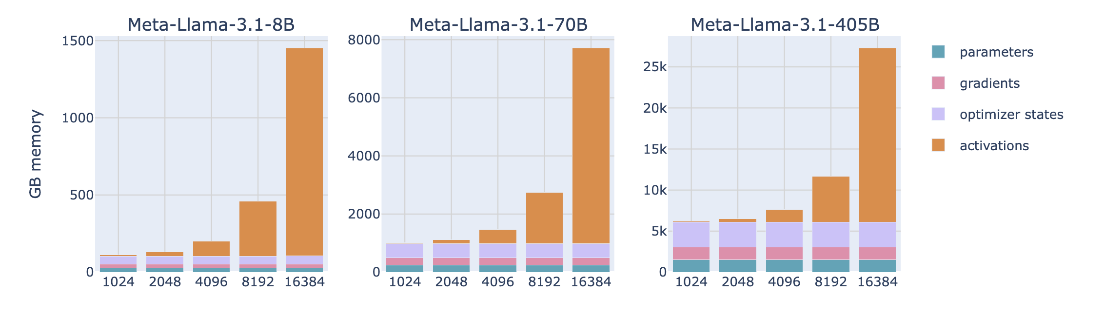
Memory for activations
- Activations stored during forward
- used to compute the gradients during backward
assuming BF16
see a previous blog for details: Memory usage - training
activations dominates memory with larger context
Memory for others
- CUDA kernels typically require 1-2 GB
- some fragamented memory cannot be used
2. How to save memory
2.1 Selective activations
aka activation recomputation / gradient checkpointing / rematerialization
https://arxiv.org/abs/2205.05198
- discared quadratic attention activations (which are very large) and re-calculate them during the backward pass
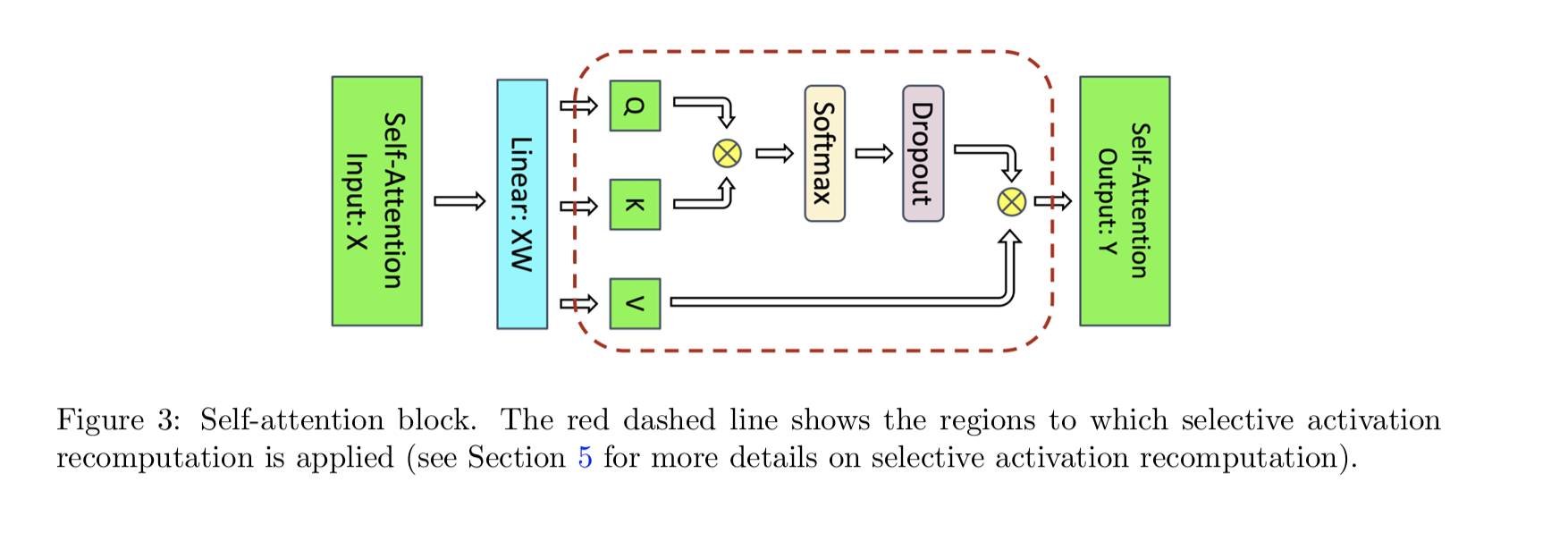
- For a GPT-3 (175B) model, this means a 70% activation memory reduction at a 2.7% compute cost
- All distributed libraries use it now, and it’s in FlashAttention
2.2 Gradient accumulation
- split a batch into micro-batches (reduce memory)
- forward and backward on each micro-batch
: micro-batch size
- compute avg gradients of all micro-batches before optimization step
: global batch size (sum of ). overall batch size between optization steps
- tradeoff between FLOPs and memory
- pros: constant memory regards of gbs
- cons: slower training (multiple foward/backward passes for one optimization step)
- difference micro-batch can run in parallel on multiple GPUs
2. Data parallelism (DP)
- Each GPU sees a different chunk (or batch) of data in parallel
- We compute the avg gradients (AllReduce) among GPUs (DP ranks)
/image.png)
- AllReduce here doesn’t overlap with any compuations → very inefficient
1. Overlap gradient sync w/ backward
/image%201.png)
- once we have calculated the gradients of one layer, we can AllReduce it
- in the meanwhile, we can calculate the gradients of the previous layer
- drawback: many AllReducd collectives are triggered, and each one has its base latency (white bubbles btw purple cells) → can be addressed by bucketing gradients
2. Bucketing gradients
/image%202.png)
- don’t do AllReduce for single gradient. we can bucket multiple gradients before each AllReduce
- default DDP bucket size is 25 MB
3. DP + gradient accumulation
- gradient accumulation: multiple forward and backward passes before updating the parameters with
optimizer.step() - DP + gradient accumulation: only a single reduce after the final step (not every backward)
- this can be done by adding a
model.no_sync()decorator
- this can be done by adding a
4. Revisiting global batch size
- mbs: the batch size seen by each GPU at a training step
- grad_acc: # gradient accumulation steps
- dp: # GPUs across the DP axis
- tradeoff btw grad_acc and dp: given a gbs, we usually maximize dp over grad_acc, since dp is parallel, while grad_gcc is sequential
5. Our journey up to now
- choose global bst: literature / experiments
- select seq length: literature / experiments. 2-8k tokens usually good
- find mbs: we now know gbs. we can increase local memory until OOM
- determine # GPUs for DP
6. Benchmark DP
- DP is the parallelism that takes the least # communications (only sync gradients, which can be overlapped with backward)
/image%203.png)
- as DP scales, throughput degragation is not that much (started to be bad at 256 in this benchmark)
- DP doesn’t change mbs, and thus memory usage is constant
up to now, we assume model can fit into one GPU, but usually it’s not → we need other parallelism
7. ZeRO (Zero Redundancy Optimizer)
ZeRO partitions optimizer states, gradients, and parameters across the DP dimension
- ZeRO-1: optimizer state partitioning
- ZeRO-2: optimizer state + gradient partitioning
- ZeRO-3: optimizer state + gradient + parameter partitioning
why activation cannot be sharded?
- each DP replica gets a different micro-batch → activations are different
Memory usage
/image%204.png)
: BF16 model param + BF16 gradients
- backward pass with the same full weights on each replica w/ different micro-batches
- w/o gradient accumulation, k = 12 (FP32 model param + FP32 Momentum + FP32 Variance)
- w/ gradient accumulation, k = 16 (k = 12 case + FP32 gradients)
ZeRO-1 optimizer state partitioning
/image%205.png)
- forward pass with full BF16 weights on each replica w/ different micro-batches
- ReduceScatter on gradients
- each replica optimize its local 1/N_d optimizer state, and gets 1/N_d FP32 weights updated, and convert to 1/N_d BF16 updated weights
- AllGather BF16 weights
/image%206.png)
how to overlap the new AllGather with computation?
- during the optimizer step: initiate the AllGather right after the optimizer updates the first slice of params
- during the forward pass: overlap AllGather of each layer’s params with the forward pass
- these techniques are not easy to implement (many hooks/bucketing)
ZeRO-2: add gradient partitioning
/image%207.png)
- AllReduce takes twice the time as ReduceScatter. Use ReduceScatter when possible.
- ZeRO-2 is always better than ZeRO-1 → you don’t have to store the weights that you don’t use for the optimizer step.
/image%208.png)
ZeRO-3: Add parameter partitioning (FSDP)
FSDP is the most popular one. It is like offloading to other GPUs.
Need to AllGather weights on demand (layer-by-layer) during forward pass
/image%209.png)
Backward pass: AllGather weights, Reduce-scatter gradients
/image%2010.png)
total communication cost of 3Ψ compared to 2Ψ for ZeRO-2
- AllGather weights during forward: communitation tax is Ψ. then discard them on the fly
- AllGather weights during backward again: communitation = Ψ
- 3Ψ is not a very big deal: we can prefetch the next layer when computing the current layer
- need to tune prefecting size (FSDP unit)
memory =
/image%2011.png)
FSDP vs TP:
- In TP, model is always shared. In FSDP, model is AllGather-ed.
- FSDP doen’t requires code changes for the model, while you must ensure correctness when adapting your code to TP.
Pros and Cons for DDP / ZeRO
- pros
- scale throughput significantly with more DP
- ZeRO: can hold larger model with sharding
- limitations
- DP assumes model can fit into one GPU
- ZeRO cannot shard activations → OOM with large seq length
- if we use activation recomputation, the activations part will go down
/image%2012.png)
3. Tensor parallelism (TP)
TP
- shard params, gradients, optimizer states, AND activations
- no communication of model params
1. Building blocks
mathematical properties
column-wise weight sharding = X broadcast + Y all-gather
/f21a3a90-ff33-4d6f-8d99-1e20a5bb1614.png)
row-wise weight sharding = X scatter + Y all-reduce
/image.png)
2. Transformer Block w/ TP
Transoform Block = Attention Block + MLP Block
MLP
TP for MLP = cloumn-wise W1 + row-wise @W2
/image%201.png)
Communication for MLP blocks
/e4047cf6-1f74-41e2-a143-7b45516bfbc1.png)
- AR must be performed before LayerNorm
- This is the implementation in Nanotron. There can be better ones with more compute-communication overlaps (check Deepseek’s async TP and DeepGEMM)
Attention
TP for Attention = column-wise for heads + row-wise for Z
/image%202.png)
- TP degree should not exceed
num_attention_heads→ it’s usally a factor ofnum_attention_heads - With GQA where
num_attention_heads>num_kv_heads, we can still set TP degree tonum_attention_heads, but needs kv heads synced properly across TP workers. - Latest LLMs don’t use Dropout anymore
TP has heavy communication
- TP does reduce activations on each device, but we need to get full activations for LayerNorm and Dropout
- TP introduces heavy communications. AllReduce cannot be overlapped → it’s in the critical path
- critical path: the sequence of ops determing the min forward time
Tradeoff: throughput vs batch size
/image%203.png)
- TP↑ means throughput↓ and batch size↑
- on NV GPU, throughput drops significantly when TP>8 (i.e., beyond one node)
TP + SP (sequence parallelism)
TP can handle Attention Region and MLP Region. How about the region between these two?
in TP, LayerNorm and Dropout need full activations
- where
and are computed across hidden dimension
- where
SP can handle it by spliting the seq dimension (rather than the hidden dimention in TP)
- the term “SP” is overloadded. in some other context, it refers to the RingAttetion that reducdes attention overheads for long context (i.e., context parallelism)
TP collectives
the figure blow shows the differences btw TP and TP+SP
/image%204.png)
- TP Foward
- f is no-op (acitvations already duplicated)
- f* is all-reduce (row linear for activations)
- TP Backward
- f* is no-op (gradients already duplicated)
- f is all-reduce (row linear for gradients)
- f and f* are conjugate pairs: when one is no-op, the other is all-reduce
- conjugate pairs: no-op ↔ allreduce and allgather ↔ reducescatter
- TP Foward
TP + SP collectives
SP replaces all-reduce with seprate all-gather and reduce-scatter
/image%205.png)
- Initial LayerNorm SP: already split by seq dimension
- SP → TP: g is all-gather for Y1 and Y2
- TP region: column linear to get W1 and W2. no communications
- TP → SP: g* reduce-scatter. reduce is to combine activations. scatter is to split by row
/image%206.png)
SP reduces the maximum activation size we need to store
- either seq or hidden is split
- activation memory is
- Q: when doing the first transition SP -> TP, we need g operation to all-gather Y1 and Y2. at this moment, the actiavtion shape is [b, s, h]. why the peak memory is not [b, s, h]
- stored vs. transient Memory
- TP: The input to LayerNorm is [b, s, h]. Because these layers happen before the split, this massive tensor must be saved (stored) in memory for the duration of the forward pass so it can be used to calculate gradients during the backward pass.
- In SP: The LayerNorm and Dropout happen on sharded data
. Only this smaller sharded tensor is stored for the backward pass.
- tiled matmul (managing the peak)
- Even for that transient “scratch” memory, modern implementations (like those in Nanotron or Megatron-Core) often don’t materialize the full [b, s, h] tensor at once → they can do tiling
- stored vs. transient Memory
Summary
| Region | TP only | TP with SP |
|---|---|---|
| Enter TP (column-linear) | h: sharded weight_out |
|
| s: full | h: sharded weight_out |
|
| s: all-gather to full | ||
| TP region | h: sharded | |
| s: full | h: sharded | |
| s: full | ||
| Exit TP (row-linear) | h: full (weight_out is full + all-reduce for correctness) |
|
| s: full | h: full (weight_out is full + reduce-scatter for correctness) |
|
| s: reduce-scatter to sharded | ||
| SP region | h: full | |
| s: full | h: full | |
| s: sharded |
And for the embedding layer:
| Region | TP only | TP with SP |
|---|---|---|
| Embedding layer (row-linear, sharded on vocab) | h: full (weight_out is full + all-reduce) |
|
| s: full | h: full (weight_out full + reduce-scatter) |
|
| s: reduce-scatter to sharded |
Limitations of TP + SP
- if seq length is too long, even with TP=8, it can still OOM → CP
- if model cannot fit w/ TP=8, there will be massive inter-node commus → PP
4. Context parallelism (CP)
- CP is similar to SP, but it applies inside the TP region
- CP doesn’t affect MLP and LayerNorm modules, where each token is processed independently
- CP does affect Attention Block → each token needs to access key/value from all previous tokens → huge communications
- Ring Attention can reduce the communication overhead
Ring Attention
https://arxiv.org/abs/2310.01889
High-level idea
- each GPU (async) send key/value to the next GPU
- while waiting for other GPUs data, it computes the attention for the data it already has
Steps (example of 4 GPUs)
GPU_i keeps
when GPU_i receives
- shape is
- shape is
- shape is
is accumulated among different pairs
- shape is
/image.png)
/image%201.png)
/image%202.png)
/image%203.png)
Zig-Zag Ring Attention
Balance # FLOPs per GPU (# cells per color is the same)
/image%204.png)
overlap: all-gather vs all2all
- Using attention as an example, but generally applied to comupte communication overlap
- Naive attention: needs to all-gather all K/V
- simpler to implement
- all-gather collective is more optimized than all2ll (which requires p2p send/received commucaiton), unless you imlement your own NCCL
/image%205.png)
- Ring Attention with all2all
- more memory efficient
/image%206.png)
5. Pipeline parallelism (PP)
- SP and CP help reduce activataions memory for long sequence.
- But they does help if model weights are too large → PP can help
- PP doesn’t save any activations memory (similar to FSDP)
- PP shard among layers
- PP need least # collectives
AFAB schedule
AFAB is for “All Forward, All Backward”: we finished all forward before doing backward
Large bubbles (device idle time)
/image.png)
let
- for the image above, imagine all computations are move to GPU1, then GPU2, 3, and 4 are all idle
- bubble ratio =
multiple micro-batches
use multiple micro-batches to reduce bubble (8 micro-batches below)
/image%201.png)
1F1B
- once a micro-batch finishes forward, it starts backward right away
- GPU4 in this example is always 1 forward + 1 backward pattern
- this way, we can release the activation memory sooner
/image%202.png)
bubble ratio remains
interleaving stages
- this introcudes more communication ops to reduce bubble time → tradeoff between commucation and bubble
- we introduce two stages: the 1st stage for the 1st half layers, and the 2nd stage for the 2nd half layers
- steps: foward for the 1st stage → forward for the 2ed stage → backward for the 1st stage. at the same time, kick off the next forward for the 1st stage → …
- this way, forward / backward for different stages can be better overlapped
/image%203.png)
- let
be the number of stages
- “Breadth-First Pipeline Parallelism” paper: there is a tradeoff btw prioritizing later stages of earlier micro-batches (depth-first) vs prioritizing early stages of later micro-batches (breath-first)
deepseek DualPipe
- DeepSeek-V3/R1 introduced a “zero-bubble” technique
- prior work: “Zero Bubble Pipeline Parallelism” paper from Sea AI Lab
- finer-grained interleaving
/image%204.png)
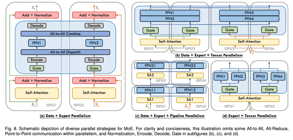
6. Expert parallelism
parallelize experts among GPUs
all-to-all operation to dispatch and collect tokens
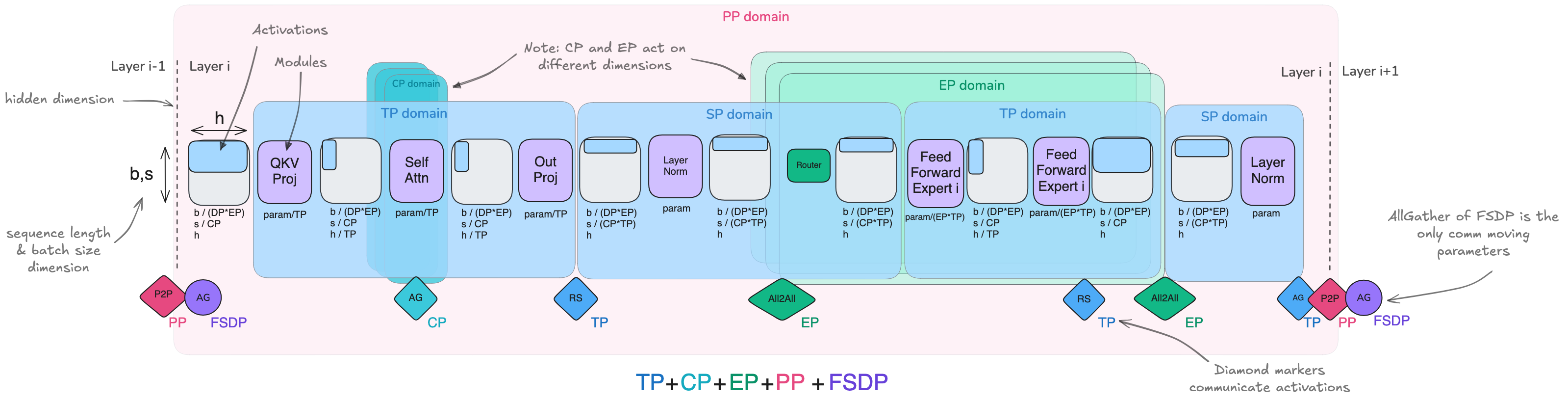
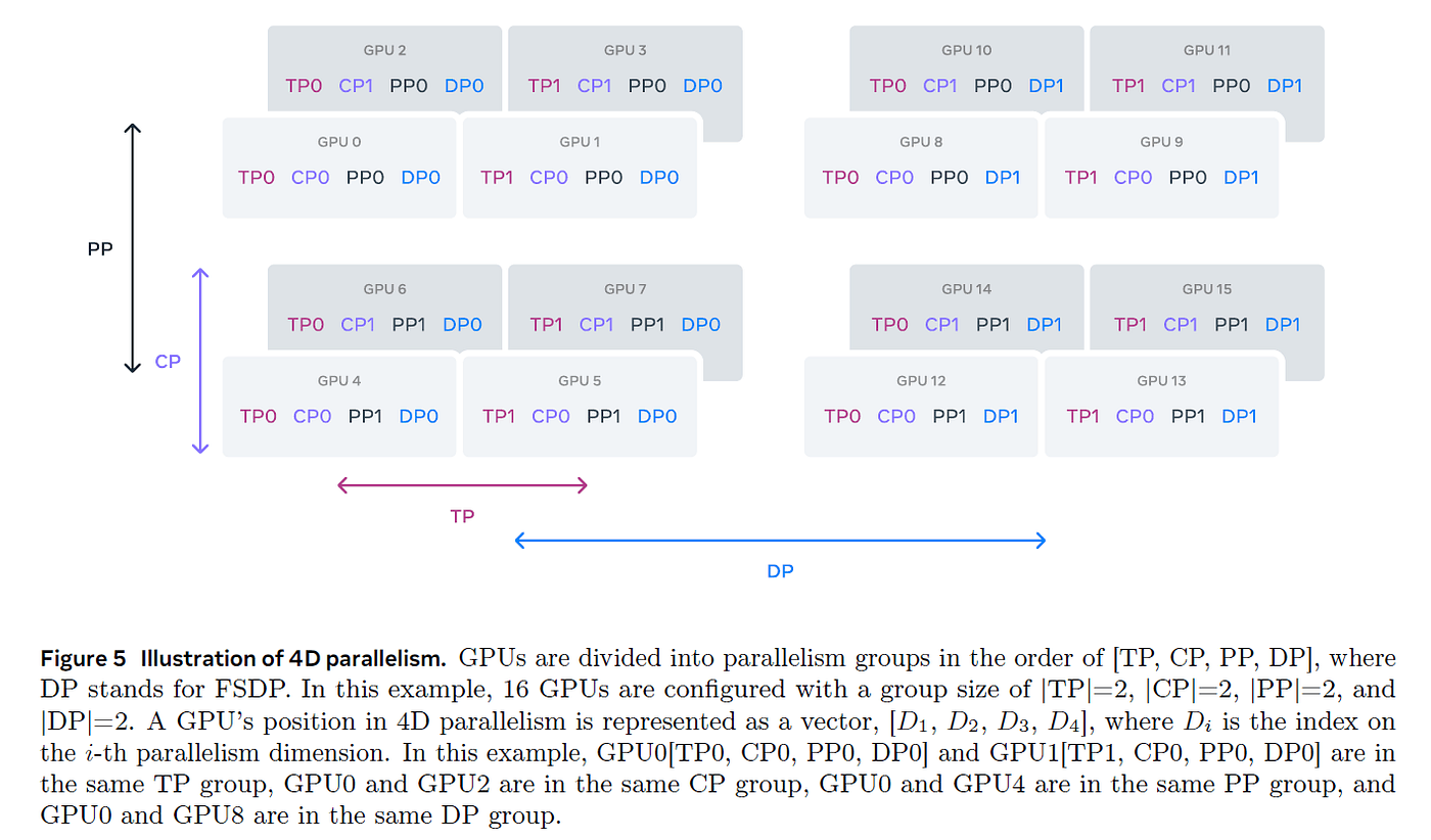
7. summary: 5D parallelism
DP: shard batch
- ZeRO-1: shard optimizer states among DP
- ZeRO-2: shard optimizer states + gradients among DP
- ZeRO-3: shard optimizer states + gradients + params among DP
TP: shard hidden
SP: shard sequence for LayerNorm; CP: shard sequence for Attention
PP: shard layers
EP: shard experts
Each parallelism operates on a different set of GPUs (different axises)
Axises are independant unless you have EP coupled with DP
ZeRO-3 vs PP
| ZeRO-3 | PP | |
|---|---|---|
| each unit stores… | only a fraction of a layer | a full layer |
| communication is used to transfer… | weights | activations |
| scaling | prefer large mb and seq_len (computes) to hide commus | prefer large gradient accumulation stepsto hide bubble |
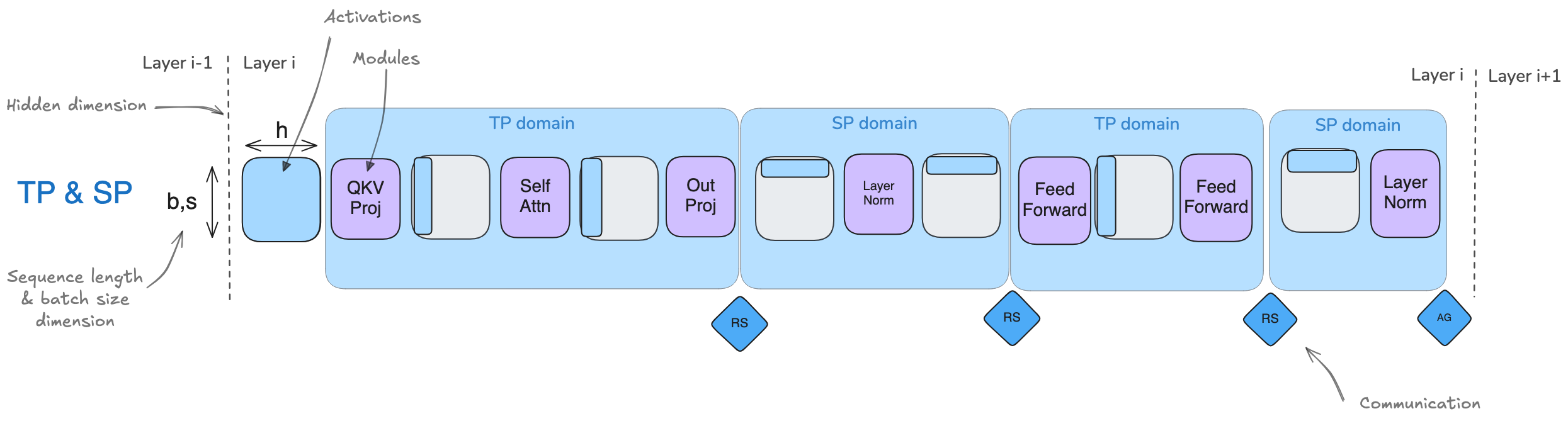
TP with SP
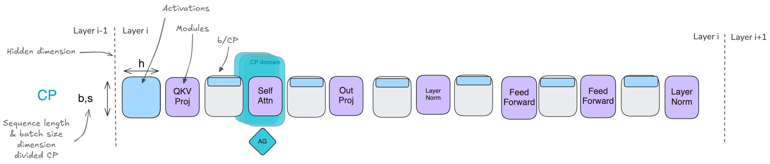
CP
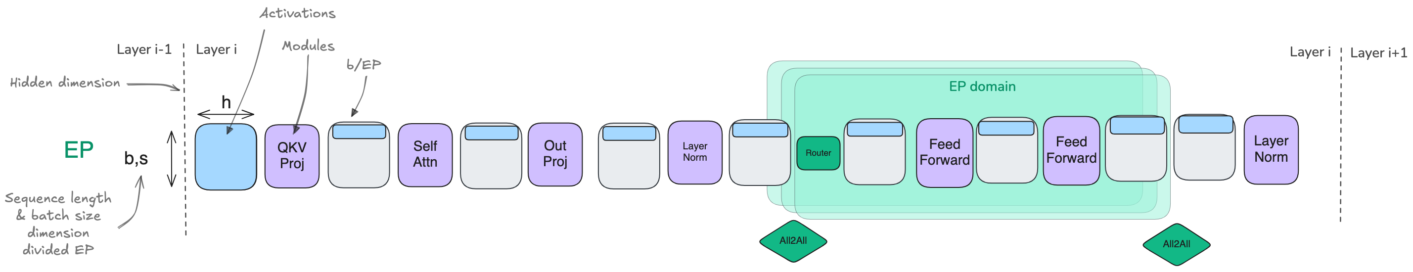
EP
5D parallelism